When you combine all of your data together in a single worksheet, you may want to verify that you do not have any duplicates.

For example, if you have combined lists of names and addresses, you want to ensure that the names are unique or only listed once.

Or you have a list of invoices and you want to make sure there are no duplicates.

Instead of manually looking through your data, use the Conditional Formatting Duplicate Values feature to get Excel to find the duplicates for you. Then you can decide how you want to handle the duplicates.

To Highlight Duplicates in Excel:

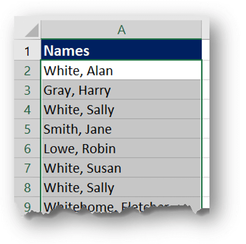
Select the range of cells you wish to check for duplicates

e.g. On sheet 1, select all of the names in your list,
select cells A2 to A400 

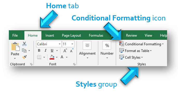
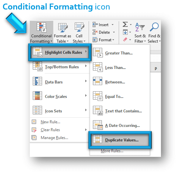
On the Home tab, in the Styles group, click the Conditional Formatting icon, choose Highlight Cells Rules, then choose Duplicate Values…

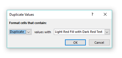
In the Duplicate Values dialog box, choose how you want the duplicate values to be formatted or highlighted.

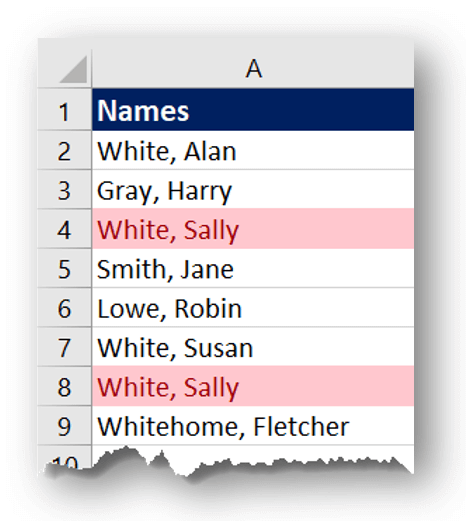
e.g. Format the Duplicate values with Light Red Fill with Dark Red Text

In our example, the Duplicate Values are highlighted according to the chosen formatting.

The Conditional Formatting Duplicate Values feature saves you from manually looking through your list for duplicates.

Please share this with other Excel users and save them hours of manual work.