Do your Column or Row Headings disappear when you scroll in your Excel worksheet?

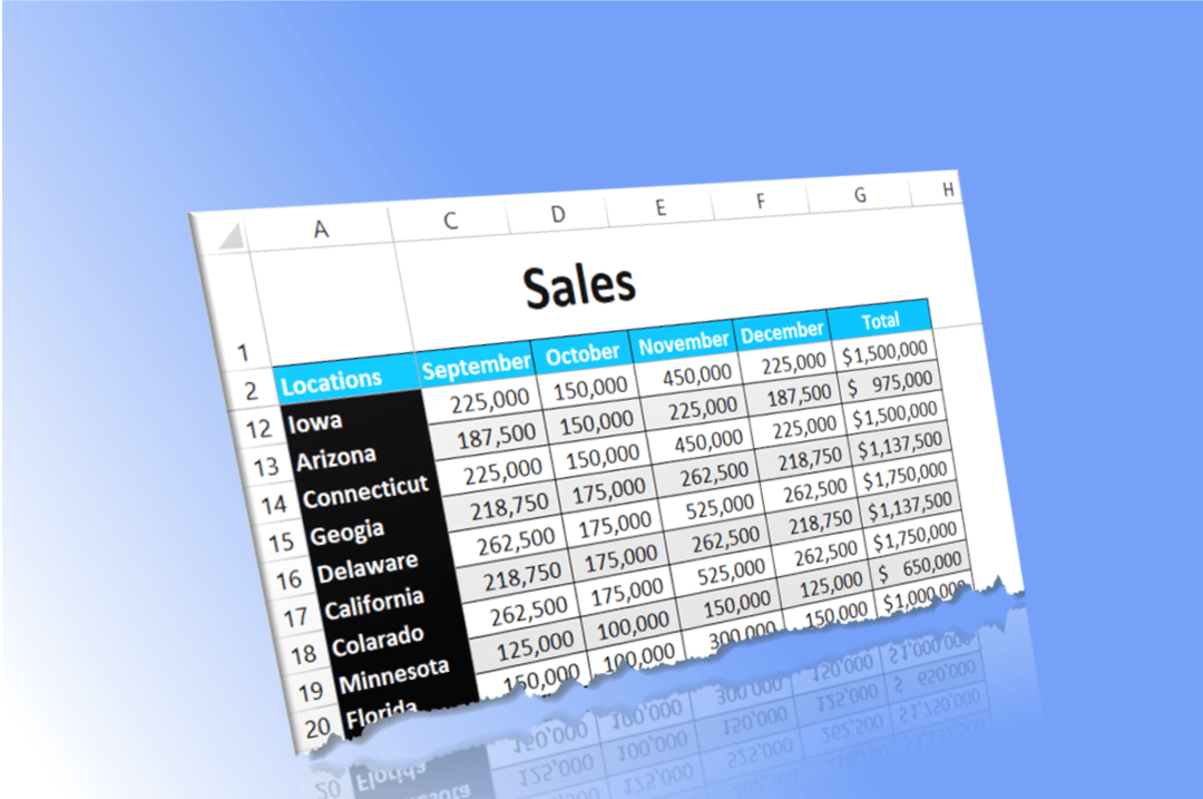
As a spreadsheet grows in size, the headings disappear as you scroll down (or to the right). Instead of repeatedly scrolling up and down or left or right to view these headings, use the Freeze Panes feature.

The Freeze Pane feature locks the Column or Row so the headings remain visible no matter where you scroll in the worksheet.

In a large spreadsheet (as shown below), the headings – Locations, Jan, Feb, Mar, Total are no longer visible as you scroll down the worksheet.

Jan, Feb, and Mar describe what the numbers in each column represent. These headings need to be visible when entering the sales for each month, as well as when analyzing and interpreting the numbers for each location.

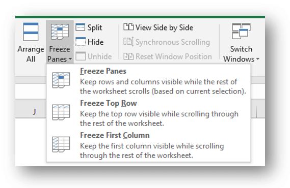
The Freeze Pane feature in Excel allows you to lock the top row(s) or left-most column(s) so your headings always remain visible while you move to different areas of your worksheet.

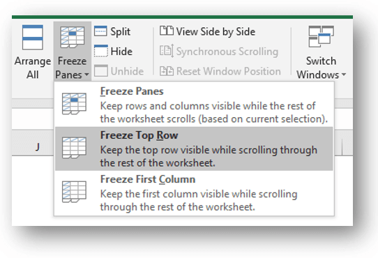
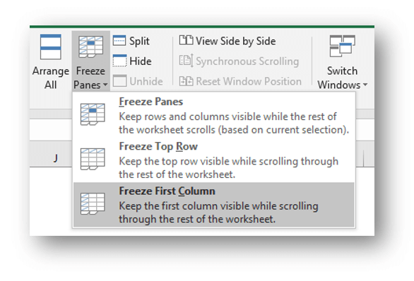
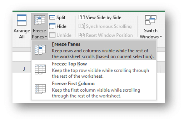
3 options are available for Freeze Panes:

* Freeze Panes

* Freeze Top Row

* Freeze First Column

How to Freeze the Top Row:

Does the first row of your worksheet contain a Heading or Title to describe the data in that column?

If yes, use Freeze Top Row.

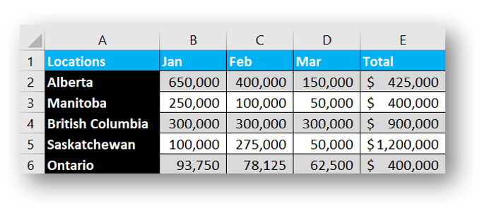
In our example, the headings are in Row 1 or the Top Row; therefore, the Freeze Top Row feature is used to lock the headings in the worksheet. When scrolling down, the headings (Locations, Jan, Feb, Mar, Total) remain visible.

Press Ctrl + Home to move to cell A1 (the top of your worksheet).
Your headings must be visible prior to moving to the next step.

On the View tab, in the Window group, click Freeze Panes, Freeze Top Row.

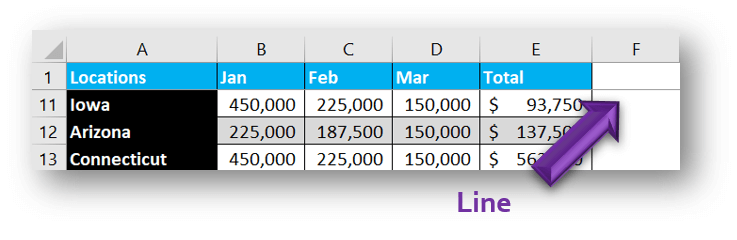
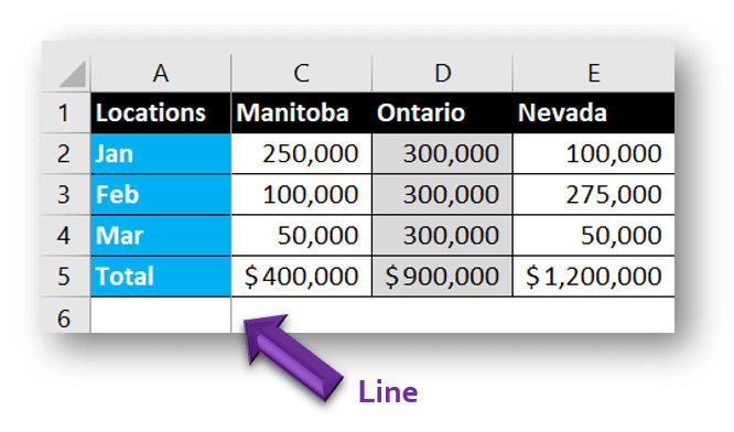
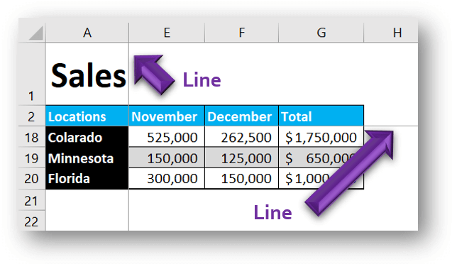
A line displays under the Top Row to indicate that it is frozen.

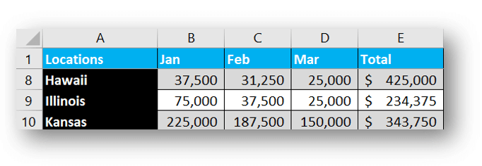
In our example, the headings in row 1 remain frozen as you scroll down to view the data in rows 11, 12, and 13.

Note: The Freeze Top Row feature freezes the top row that is displayed.

For example, if Row 10 is the Top Row displayed in your worksheet, Row 10 is the row that is locked.

Recommendation: Press Ctrl + Home prior to using the Freeze Top Row feature.

Note: When you freeze a worksheet, it has no effect on how the worksheet is printed.

How to Freeze the First Column:

Does the first column of your worksheet contain a Heading or Title to describe the data in that row?

If yes, use Freeze First Column.

In our example, the headings are in Column A or the First Column; therefore, the Freeze First Column feature is used to lock the headings in this worksheet. When you scroll to the right, the headings (Locations, Jan, Feb, Mar, Total) remain visible.

Press Ctrl + Home to move to cell A1 (the top left corner of your worksheet).
Your headings must be visible prior to moving to the next step.

On the View tab, in the Window group, click Freeze Panes, Freeze First Column.

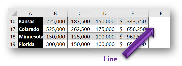
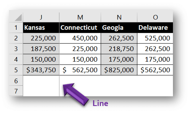
A line displays beside the First Column to indicate that it is frozen.

In our example, the headings in column A remain frozen as you scroll right to view the data in columns C, D, and E.

Note: The Freeze First Column feature freezes the First Column that is displayed.

For example, if Column J was the First Column displayed in your worksheet, Column J would be locked.

Recommendation: Press Ctrl + Home prior to using the Freeze First Column feature.

Note: When you freeze a worksheet, it has no effect on how the worksheet is printed.

How to Freeze More than One Row or Column Heading:

Do you have more than one Row or Column that contains a Heading or Title?

Or do you want both the Row and the Column Headings to be frozen at the same time?

If yes, use Freeze Panes.

To use the Freeze Panes feature, you must select an Anchor Cell.

All rows above the Anchor Cell will remain visible while scrolling.

All columns to the left of the Anchor Cell will remain visible while scrolling.

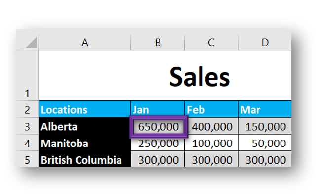
In our example, you may wish to lock the Months (in Row 2) and the Locations (in Column A). Therefore, as you Enter or Analyze the data, the Months and Locations remain visible if you scrolled down or to the right.

In order to freeze these rows and column, the Anchor Cell must be Cell B3.

Go to the Anchor Cell.

* All rows Above the Anchor Cell will be frozen.

* All columns to the Left the Anchor Cell will be frozen.

On the View tab, in the Window group, click Freeze Panes, Freeze Panes.

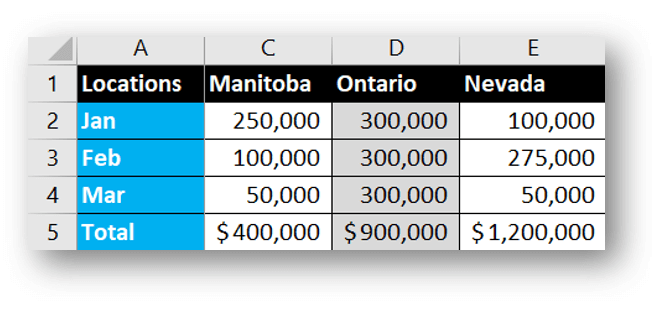
Now all rows above Row 2 are frozen and all columns to the left of Column B are frozen. As you Enter the Sales figures, both the Month and the Location remain visible.

A line displays to indicate the frozen rows and columns.

Note: When you freeze a worksheet, it has no effect on how the worksheet is printed.

How to Modify Freeze Panes / Unlock the Row or Column (or Clear Freeze Panes):

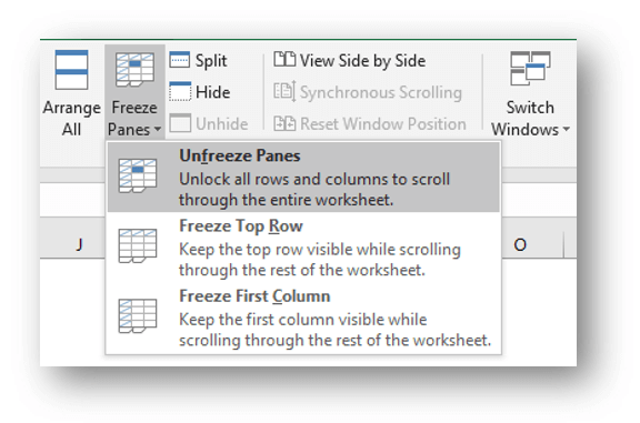
Do you want to modify what Rows or Columns are frozen? If yes, use the Unfreeze Panes feature. Then use the Freeze Top Row, Freeze First Column, or Freeze Panes to lock the correct headings.

Do you want to turn the Freeze Panes feature off? If yes, use Unfreeze Panes.

On the View tab, in the Window group, click Freeze Panes, Unfreeze Panes.

The Row or Column headings are no longer locked. As you move through your large spreadsheet, the headings disappear.

Note: the UnFreeze Panes feature is only available if the one of the Freeze Panes options has been used on the worksheet.

* Freeze Panes

* Freeze Top Row

* Freeze First Column 

Tables and Freeze Panes

Note: If you have used the Format as Table feature, you may not need to use Freeze Panes. Excel automatically displays the column headings when you scroll down.

However, if you want to lock specific columns and rows, use the Freeze Panes feature.

Freeze Panes – Keyboard Shortcut

In Excel, press and release the Alt key to display key tips for each tab in the Ribbon.

Press the letter corresponding to the specific Ribbon tab to display the shortcut key for all of the commands on that tab.

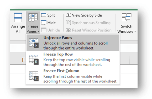
Press Alt + W, F, and then press the specific letter to choose one of the Freeze Pane features.

* F = Freeze Panes or Unfreeze Panes

* R = Freeze Top Row

* C = Freeze First Column

Please share this with other Excel users and help them work with large spreadsheets.